From “will it route” to “will it work”: electrical analysis drives layout

In the last article we described DeepRoute, the tournament router inside PackageCompiler. This is the second of the three, and it is about the electrical analysis. We promised an electromagnetic engine that lives inside the router instead of down the hall. Putting it there buys two things. The obvious one is turnaround: an answer in the same compile, not next week. The one that matters more is that the analysis can drive the layout. Physical synthesis guided by electromagnetic analysis becomes possible, and that is the theme of everything below.

The analysis lives where the geometry lives. In a conventional flow the router and the field solver are different products, often from different companies. You route, export, import into the solver, wait, read a report, and carry the findings back by hand. Every hop is a translation, and analysis becomes a milestone that costs project a week per iteration.

In PackageCompiler the analysis is code in the same binary as the router, and it reads the same in-memory geometry the router wrote: the netlist, the routed wires, the poured planes and the padstacks the via placer minted, with no export and no import. The stackup, the materials and the design rules come from the one PDK that drives routing and DRC, so the width the analysis measures is the width the router drew, under the plane that was actually poured. Three things follow. The analysis runs on every compile, because the cheap tier costs microseconds per trace. The report describes what was built, not what was intended. And a number the analysis computes can flow back into the router as a constraint: when analysis and synthesis share a codebase, the distance between a report and a rule is one function call.

When the data is missing, the report says so. A stackup with no dielectric, a material with no loss tangent, a trace with no reference plane: each is a gap in the input, and the analysis reports the gap rather than hallucinating a number to fill it. Every row names the tier that produced it and what that tier cannot see, so a number is never more confident than the data behind it.

What runs, and what it changes. For each analysis, the question that matters is whether it only reports, or whether it shapes the route.

Traces. Three tiers read the same geometry: closed-form formulas in microseconds, a 2D field solve in about a second per distinct cross-section, and a full-wave 3D solve in minutes for a handful of named nets. The report gives impedance, delay and loss per wire section, flags any section or whole net whose delay exceeds a sixth of the rise time for termination, and verifies each differential pair’s skew, coupling and differential impedance. The impedance shapes the route: you give a target, the compiler inverts the line model for each layer’s stack, and the router widens every trace to that width the moment it is clear of the bump field. So does length matching, which splices a meander into the shorter leg of a pair.

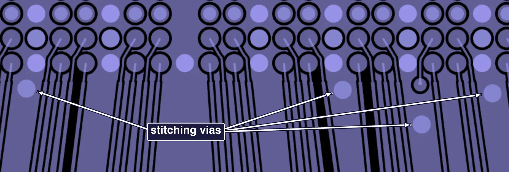
A corner of the E6 bump field on CU1, straight from a compile. Each trace leaves its pad at the width the bump pitch allows and steps up to the 50 Ω width as soon as it is clear of the pads; the impedance report carries both halves as separate rows, 66 Ω for the neck and 50 Ω for the run. The marked discs are stitching vias tying the ground fill to the plane beneath, and their spacing is set by the signal, not by hand: a 100 ps edge has a knee frequency of 3.5 GHz, whose wavelength in this 3.4 laminate is 46 mm, and the fill is gridded at a twentieth of that, 2.3 mm. Two rules then add vias where the grid alone would leave a gap. Every fragment of fill that the escape traces slice off gets at least one via of its own, which is why the vias here sit far closer than the grid pitch, and every signal via that changes layer gets a return via within 1 mm, like the one directly below the signal via at the right.

Crosstalk. The designer declares a budget, the near-end crosstalk a sensitive net may receive from one neighbour, and the compiler solves the coupled pair for each layer and turns it into an edge-to-edge spacing per net that the router honours in both global and detail routing. The report then measures what was delivered, per victim and aggressor. Shapes the route.

Vias and return paths. Every layer change is read from its padstack, grouped into classes (two thousand vias is typically about ten distinct structures), field-solved once into a two-port model, and composed with the trace sections into the net’s end-to-end response; a geometric screen flags via stubs that resonate in band. Where a trace leaves the copper it is referenced to, the break is found, classified and measured, and the crossings that repeat get a small library of their own. Report.

Stitching vias. The return path is not only checked; it is built. Ground fills and planes are stitched at a pitch set by the signal’s knee frequency, a twentieth of a wavelength, with plane-to-plane columns placed before routing so the router treats them as obstacles, and a return via beside every signal via that changes layer. Shapes the route.

Power. Each power net’s planes, vias, balls and bumps are solved as one resistive network, giving the drop at every bump, the current through every via and the ground rise at the die, with a 3D view of the copper coloured by drop. Report, today. Plane connectivity is the other half: a net poured on two layers is one net only if something joins them, and the compiler detects planes that nothing spans and builds the columns, ball by ball. Shapes the route.

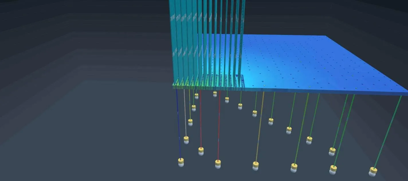
One VDDC quadrant of E6: the plane, the column of bump vias rising to the die, and the ball columns hanging below it, each via coloured by the DC current it carries. The two red columns exceed the copper’s current-density limit in the PDK. Columns below the display threshold are greyed out.

So the split today: impedance sets widths, crosstalk sets spacings, stitching and plane columns are constructed, pairs are length-matched. Vias, return-path breaks, termination and DC drop are reported with the evidence attached and left to the designer.

Where this goes. The next step is the obvious one: the rest of the list moves from the report into the route. A via that resonates in band should be back-drilled or made blind by the via placer, not flagged. A return-path break should cost the router something before the wire is committed. The DC drop map should feed the ball assignment and the plane strategy, so power balls land where the current wants to go. And the electrical results should join the tournament’s score, so a configuration that routes cleanly but rings loses to one that routes cleanly and works.

That is the arc of the series. The first article was about a router that asks “will it route” of thousands of candidates and keeps the best. This one is about the analysis that asks “will it work”, built close enough to the router to answer on every compile. The work ahead is to let the second question drive the first.